Topocurrencies : quand l'argent apprend où il se trouve

L'argent a toujours été spatial

Chaque pièce de monnaie jamais frappée vous disait où le pouvoir vivait. Les drachmes athéniennes portaient le hibou d'Athéna — dépensez ceci à portée de notre marine. La livre sterling provenait du poids en livres des pennies d'argent — la confiance mesurée en métal, limitée par la portée du souverain. Le dollar américain fonctionne parce que les porte-avions et les accords commerciaux étendent sa portée à chaque port de la Terre. L'argent a toujours été une technologie spatiale : un moyen d'encoder la confiance à travers la distance, limité par la géographie de celui qui la soutient.

Puis la cryptomonnaie a rompu le lien. Le Bitcoin ne sait pas où il se trouve. L'Ether ne se soucie pas du continent sur lequel se trouve son validateur. Pour la première fois dans l'histoire monétaire, nous avons construit des instruments financiers sans aucune conscience géographique. Ceci a été célébré comme une caractéristique — sans frontières, sans permission, indépendant de la localisation.

La première conséquence est l'inégalité spatiale structurelle. Les banques collectent des dépôts dans les communautés rurales et périphériques, puis canalisent ces dépôts dans les prêts dans les centres urbains où les valeurs des garanties sont plus élevées et les rendements plus prévisibles. Une étude de 2025 de l'American Economic Review a documenté cela directement : les banques dans les comtés plus pauvres et ruraux canalisent systématiquement les dépôts vers l'extérieur, tandis que le pouvoir du marché local a « un effet très négatif substantiel sur le flux de crédit vers les comtés plus petits/plus pauvres ».¹ Gunnar Myrdal les appelait « effets de rétraction » — les processus d'auto-renforcement par lesquels le capital financier s'écoule de la périphérie vers le centre.² Douze millions d'Américains vivent dans des déserts bancaires, 65% d'entre eux ruraux.³ L'argent crée des gagnants et des perdants spatiaux.

La deuxième conséquence est la cécité écologique. La valeur mondiale des services écosystémiques — pollinisation, purification de l'eau, séquestration du carbone, régulation des inondations — est estimée à 125-145 billions de dollars par an, rivalisant avec le PIB mondial total — un chiffre débattu en méthodologie mais directionnellement incontesté en échelle.⁴ Cependant, les services écosystémiques sont spatialement spécifiques. Une forêt de mangrove dans les Sundarbans protège Calcutta des cyclones ; elle ne fait rien pour le Kansas. Un bassin versant dans les Andes alimente les robinets de Lima ; il n'a pas de sens pour Lagos. Le schéma spatial des services écosystémiques varie de l'hyperlocal au planétaire, et l'argent actuel ne capture aucune de ces variations.

Les deux problèmes partagent une cause racine : de l'argent qui comprime loin l'information géographique. La cryptomonnaie, en effaçant la géographie entièrement, n'offre aucun remède. Une analyse de 1,84 milliard de transactions dans huit grandes cryptomonnaies a révélé que la concentration de richesse dans les marchés de cryptomonnaies reflète ou dépasse celle de la finance traditionnelle.⁵ L'argent indépendant de la localisation reproduit la cécité spatiale à la vitesse numérique.

Une topocurrency (du grec topos, lieu + currency) est une cryptomonnaie dont les propriétés — valeur, utilité, droits de gouvernance, taux d'émission ou règles de transaction — sont modifiées par programmation en fonction de la localisation géographique. Le terme est proposé ici pour un espace de conception émergeant indépendamment dans la finance spatiale, les marchés environnementaux et l'informatique spatiale. Les modèles qu'il nomme sont déjà en cours de construction.

Ce qui distingue les topocurrencies des monnaies communautaires antérieures (Ithaca Hours, Bristol Pound, Chiemgauer), c'est que la géographie elle-même devient programmable. Une topocurrency lit la région dans laquelle elle circule. Ses contrats intelligents peuvent répondre à l'état écologique d'un bassin versant, à l'intensité du carbone d'un réseau énergétique ou à l'indice de biodiversité d'une zone protégée — en ajustant les incitations en conséquence.⁶

Mais la géographie programmable nécessite une primitive technique que les blockchains actuelles n'ont pas : un moyen de vérifier, onchain, que quelque chose s'est produit à un lieu et à un moment spécifiques.

---

Preuves de localisation

Faire de l'argent qui sait où il se trouve nécessite une primitive : la preuve de localisation — un artefact numérique vérifiable qui soutient une affirmation sur le calendrier et la localisation d'un événement observé. Le Berlin Token d'Astral illustre le concept à son plus élémentaire : un jeton qui ne peut être frappé ou transféré que par des personnes physiquement présentes dans une limite définie.⁷ La géographie encodée comme loi économique.

Tout système qui rend l'argent spatial a besoin d'un moyen de vérifier les affirmations de localisation sans faire confiance à une seule autorité. Several projects have attacked pieces of this — FOAM Protocol pioneered terrestrial proof-of-location beacons⁸, and Brito (2025) formalized the fault-tolerance requirements⁹ — but no complete pipeline existed until recently. Nous utilisons Astral comme notre exemple courant car il offre l'implémentation la plus mature de la pile complète : de la collecte de preuves brutes à travers la composition cryptographique à l'attestation onchain. Ce qui suit illustre l'espace de conception général à travers une architecture spécifique. Les problèmes qu'Astral résout — composition de preuves, confiance graduée, confidentialité, calcul vérifiable — sont les problèmes que tout système de preuve de localisation doit résoudre.

Architecture de la preuve de localisation d'Astral

Astral’s framework defines three components:⁷

• Location Claims — spatially-referenced assertions. Claims describe areas (not points), with a mandatory radius parameter and temporal bounds. A claim says: “this entity was within this area during this time window.”
• Location Stamps — independent pieces of evidence. Device attestation (ProofMode), infrastructure verification (WitnessChain), GPS readings, Wi-Fi signatures, Bluetooth beacons, cell tower triangulation, signed attestations from nearby devices. Each stamp is independent of any claim — raw evidence, not assertions.
• Location Proofs — bundles of stamps with a claim. When verified, they produce a multidimensional CredibilityVector — evaluating location evidence across independent dimensions (spatial accuracy, temporal alignment, stamp validity, and source independence). Different applications weight these dimensions differently; a weighting function can collapse the vector into a single CredibilityAssessment score that contracts can threshold against, but the vector itself is the richer, more informative artifact.

The security model relies on independence: a single stamp can be forged, but forging two or three unrelated stamps simultaneously is substantially harder. Correlated evidence — multiple GPS readings from the same device, for instance — adds little, because compromising one compromises all.¹⁰

Location stamps draw from seven categories of evidence:¹⁰

Table 1: Location proof evidence categories and forgery resistance.

Category	Example	Forgery Difficulty
Authority	Government-issued survey markers	High (institutional trust)
Social	Attestation from known local residents	Medium (collusion possible)
Near-field machine	Bluetooth/NFC beacon handshake	Medium (requires physical proximity)
Network machine	Cell tower triangulation, IP geolocation	Low-medium (network-level spoofing)
Sensor data	Barometric pressure, magnetic field, ambient sound	Medium (environmental fingerprints hard to fake)
Delegated	Third-party verification service	Varies by provider
Legal	Notarized GPS coordinates, property deed	High (legal consequences)

A robust topocurrency transaction might require stamps from at least two independent categories. A neighborhood cleanup token (low stakes) might accept a single attested check-in. A biodiversity credit worth thousands of dollars (high stakes) might demand a score above 0.9, combining satellite imagery, IoT sensor data, and social attestation from local rangers. The governing constraint: the cost of forging a location proof should exceed the economic value of the transaction it underpins.⁷

Location data is among the most sensitive data categories. ZK point-in-polygon proofs — demonstrated by ZKMaps and formalized in IEEE research on floating-point SNARKs for geographic region proofs¹¹ — let users prove they are inside a geographic boundary without revealing exact coordinates. Astral’s documentation makes a crucial distinction: GPS coordinates alone are just numbers — without corroborative evidence, a zero-knowledge proof over coordinates proves geometry, not location.¹⁰ Topocurrencies need both: multiple signals for verification, zero-knowledge proofs for privacy.

A critical distinction: Astral provides verifiable computation, not verifiable location.⁷ The Location Proof framework verifies that input data is honest. The Geospatial Policy Engine runs PostGIS — the standard open-source geospatial database — inside an EigenCompute Trusted Execution Environment (TEE), a hardware-isolated enclave where code executes in encrypted memory that neither the host operator nor external observers can inspect or tamper with. This proves that spatial calculations were performed correctly on honest inputs, without exposing the underlying data. The architecture has three stages: (1) Location Proofs verify that spatial data inputs are credible; (2) Geospatial Computation performs spatial operations (containment, distance, intersection) in a trusted execution environment; (3) Onchain Verification anchors results as EAS attestations that smart contracts can read and respond to. The SDK (v0.2.0) implements this as operational infrastructure, not a roadmap.

---

La pile de finance spatiale

Three technologies — programmable money (crypto), verifiable spatial data (location proofs), and autonomous economic actors (AI agents) — are each individually useful. Programmable money enables conditional and performance-based transactions, verifiable spatial data provides location-based attestations, and AI agents can process environmental data at scale. But the combination produces something qualitatively different: the ability to create money that responds to the physical world in real time.

Crypto alone reproduces the same spatial inequality as conventional finance — wealth concentrates through the same mechanisms regardless of whether the ledger is centralized or distributed. Adding location proofs gives verified spatial data, but verified location data cannot by itself create incentives or direct capital flows. And neither crypto nor spatial proofs can process planetary-scale environmental data or manage autonomous monitoring across thousands of sites — that requires AI agents.

Les agents IA comme acteurs économiques spatiaux

The Location Protocol specification explicitly envisions “localized AI agent behavior” as a use case.¹² Location proofs verify where. Crypto handles value transfer. But neither can process the planetary-scale ecological and energy data that spatial verification demands, nor manage the continuous monitoring that ecological accountability requires. AI agents close this gap — they are the operational layer that connects verified spatial data to economic action.

What location-aware AI agents enable:

• Continuous environmental monitoring — satellite imagery, sensor networks, and ecological models running MRV (Monitoring, Reporting, and Verification) at a fraction of human cost, feeding metrics directly into token issuance functions⁵⁴
• Spatial price response — agents that read real-time environmental data (grid carbon intensity, soil moisture, biodiversity indices) and route economic activity toward locations where it does the least harm
• Autonomous treasury management — allocating bioregional funds based on ecological signals: fire prevention when vegetation dries, flood mitigation when water tables rise, conservation payments when species decline
• Verifiable identity — if agents route capital and manage treasuries, the system needs to distinguish trustworthy agents from malicious ones. ERC-8004 (mainnet January 2026) establishes onchain registries for autonomous agents — identity, reputation history, and validation status — so that a topocurrency contract can set minimum reputation thresholds before granting an agent routing or allocation authority²⁷

Contrats géospatiaux : capturer l'argent existant

A topocurrency can work two ways:

1. Constrain existing money. Take an established stablecoin — USDC, USDT, or any asset with established liquidity — and lock it into a geospatial smart contract that modulates its behavior based on location. The territory “captures” external liquidity and keeps it recirculating locally.
2. Mint new tokens. Create a currency backed by verified spatial outcomes — mangrove restoration, sustained territorial presence, or service provision — where monetary supply expands in proportion to measured work.

The choice depends on the use case, but Astral’s spatial primitives make both architectures operational. A contains() check determines whether a transaction occurs within a territory’s boundaries. A distance() function modulates fees based on proximity to a resource. A within() query verifies membership in a spatial zone. These primitives execute off-chain in Astral’s Geospatial Policy Engine (PostGIS in a TEE) and their results are anchored onchain as EAS attestations that contracts can verify. Combined with environmental or economic data feeds from oracles, they turn generic value — whether captured stablecoins or freshly minted tokens — into location-aware money that responds to where it is.

Stablecoin capture matters because bootstrapping a new currency is hard. Constraining existing money requires programmable token logic — conditional holds, spatial gating, automated fee redistribution — that traditional payment rails do not expose. DeFi has already built these primitives: programmable escrow, conditional release, automated market-making, and oracle integration. A geospatial smart contract composes these with location proofs; it does not need to reinvent them. Service-backed minting matters because some territories need a currency that reflects local value creation, not just imported liquidity. The design space below maps which use cases call for which approach.

---

Le marché du calcul spatial : acheminer l'IA vers l'énergie abandonnée

Spatial compute is where the topocurrency thesis is most concrete: the market is large, the data exists, and three powerful primitives — spatial verification, oracle feeds, and programmable fee modulation — converge in a single mechanism.

The idea is simple. AI companies need enormous amounts of electricity. In some places, surplus clean energy is being thrown away because nobody is there to use it. In other places, data centers are overwhelming grids that were never built for this load. The cost difference between these locations already exists — but it is scattered across electricity tariffs, cooling engineering specs, water utility rates, and transmission congestion reports that no single actor aggregates in real time. A topocurrency does three things: it composes these cost dimensions into a single comparable signal across zones, updates that signal continuously via oracle feeds rather than annually via bilateral contracts, and provides settlement infrastructure so that agents can act on the signal immediately. The result is that flexible compute workloads route to where cheap, clean energy is abundant — saving operators money, relieving grid stress, and converting wasted generation into productive capacity. Not all compute can move — data gravity, regulatory constraints, and infrastructure requirements limit the locationally flexible fraction to roughly 10–20% of total data center energy today — but that fraction is growing as AI’s share of compute increases, and even at this smaller number the efficiency gains are substantial.

Over 100 TWh of clean energy was curtailed globally in 2024 — generation capacity that the grid could not absorb.¹³ China alone curtailed an estimated 80 TWh of wind and solar. In advanced economies the numbers are smaller but growing fast: ERCOT curtailed 8 TWh, CAISO 3.4 TWh, the UK 6.6 TWh, Germany 9.3 TWh. The problem is structural: as renewable capacity additions outpace transmission infrastructure, curtailment volumes increase alongside the installations meant to solve the climate problem.

Simultaneously, AI compute is overwhelming the grids it already sits on. PJM Interconnection’s December 2025 capacity auction closed 6,517 MW short of its reliability target, with data centers responsible for 94% of projected load growth.¹⁴ Northern Virginia alone hosts roughly 6 GW of data center capacity — approximately 13% of the global total — stressing a grid that was not built for this concentration. IEA projects global data center electricity consumption will double from 460 TWh in 2024 to 945 TWh by 2030, growing at 15% per year — four times faster than total electricity demand.¹⁵

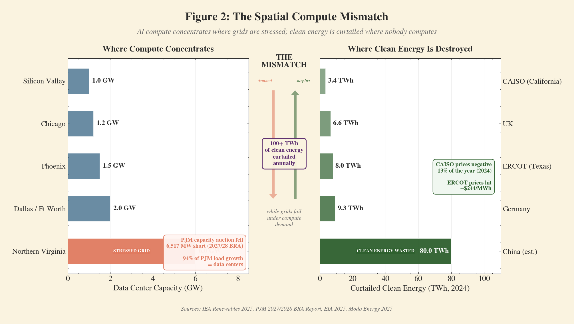
Clean energy goes uncaptured in one place because nobody is there to use it. Grid capacity fails in another because everyone concentrates in the same location. A topocurrency can address both: route locationally flexible compute toward sites with surplus clean energy, relieving grid congestion at the source and monetizing energy that would otherwise be wasted.

Pourquoi l'optimisation à une seule variable échoue

Spatial compute shifting is not hypothetical. Google and Microsoft already move workloads temporally and spatially to reduce carbon intensity — Google achieving 66% carbon-free energy hourly across its fleet since 2021, Microsoft’s Carbon-Aware SDK delivering roughly 10% emissions reductions for Azure Batch workloads.¹⁶ This proves the infrastructure works: workloads can move across regions in response to real-time signals.

But carbon is a signal that only motivates actors who already care about carbon. Most compute buyers do not — they care about cost. And carbon intensity, on its own, is a weak routing signal: Sukprasert et al. (EuroSys 2024) tested three years of hourly carbon data across 123 cloud regions and found that geographic load shifting achieves carbon reductions “of the order of 5%” — because cloud providers cluster in regions with similar grid mixes.¹⁷

The operational costs that actually determine where compute should run — energy price, cooling load, water withdrawal, grid congestion — vary far more dramatically across locations, and they vary independently of each other. The total cost differential between Iceland and Virginia is roughly 57%. Carbon intensity is one dimension of that gap; cost is the whole picture.

The electricity market already proves that spatial granularity in pricing works. Locational marginal pricing (LMP) computes approximately 11,000 location-specific prices every five minutes in PJM alone, and when ERCOT replaced a handful of regional price averages with node-level pricing — one price per grid connection point — operating costs fell 3.9%, over $300 million per year.¹⁴ A topocurrency applies the same logic to compute placement: instead of routing on carbon — a signal that reaches only the already-motivated — it routes on total cost, a signal that reaches everyone.

La topocurrency en tant que plateforme d'appariement

The spatial compute market is a matching problem, not a pricing problem.

Flexible compute demand and stranded renewable supply have complementary profiles, but connecting them efficiently requires more than a uniform price. Different compute workloads tolerate different levels of intermittency (training can be checkpointed every four hours; real-time inference cannot be interrupted). Different renewable sites have different temporal profiles (West Texas wind peaks at night; CAISO solar peaks at midday), grid connection statuses, and cooling environments. A topocurrency must match along multiple dimensions simultaneously — energy price, latency tolerance, cooling advantage, carbon intensity, water availability — not just clear a single market.

This is the structure Rochet and Tirole (2003) describe in their foundational work on two-sided platforms: an intermediary that creates value by connecting two distinct groups whose participation benefits the other side.¹⁸ Each additional flexible workload routed through the platform makes it more attractive to renewable operators (more curtailment absorbed, more revenue from stranded energy); each additional renewable site makes the platform more attractive to compute operators (more options for cheap, clean energy). Cross-side network effects drive adoption without mandates.

This is already happening ad hoc. Crusoe Energy routes compute to stranded energy sites — mitigating 2.7 million tons of CO2-equivalent emissions and, in March 2025, pivoting from Bitcoin to AI compute to capture higher revenue from flexible workloads.¹⁹ Virtual power plants aggregate distributed energy resources into dispatchable capacity: the Brattle Group (2023) estimates 60 GW of VPP deployment could meet U.S. resource adequacy needs at $15–35 billion less than conventional alternatives.¹⁹ But these are bilateral arrangements — each one negotiated individually, each limited to the participants who found each other. A topocurrency replaces bilateral negotiation with a continuous matching surface: any flexible workload can discover any available site, compare total cost across dimensions, and route in real time. The platform scales the matching, not just the price.

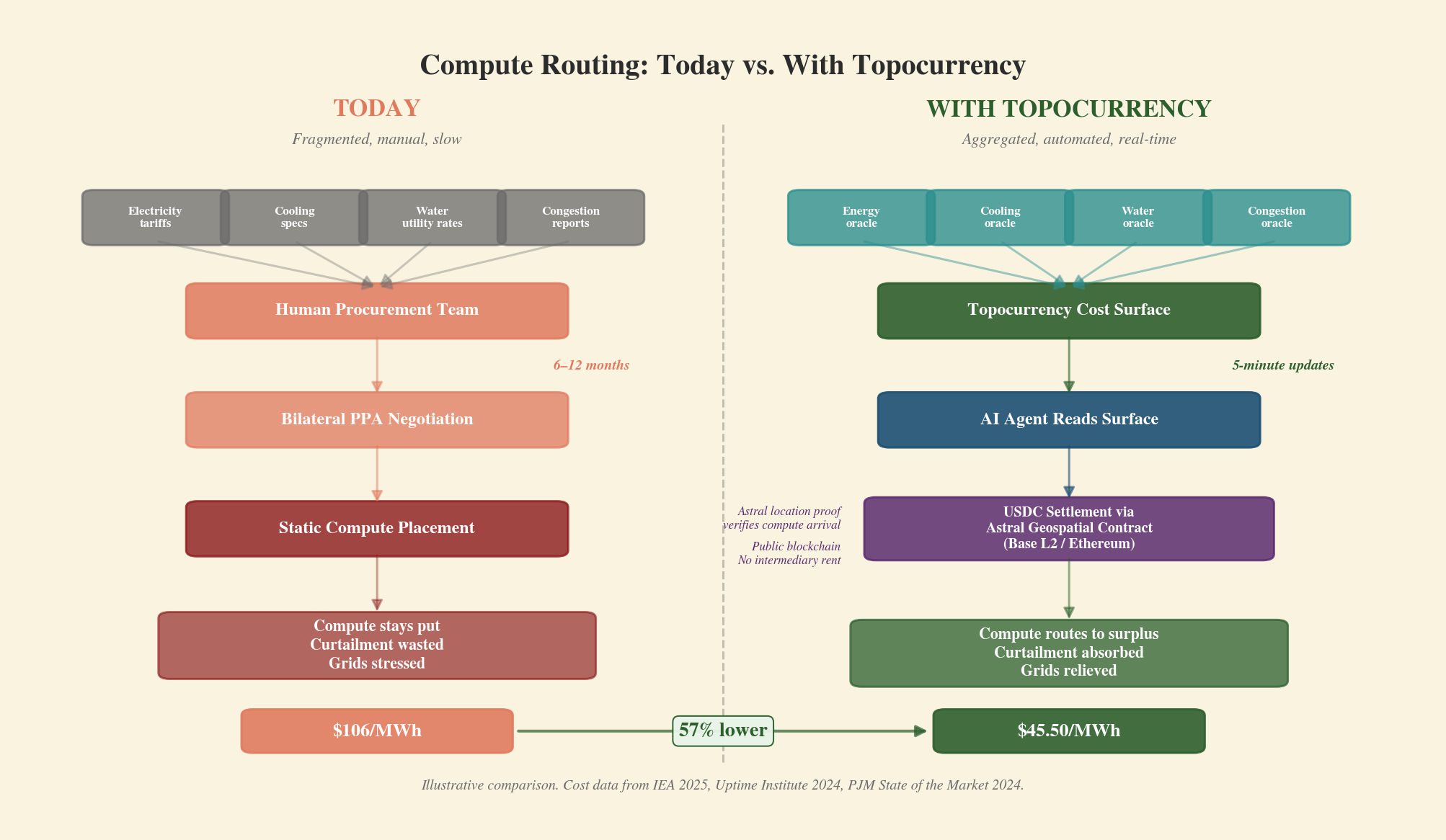
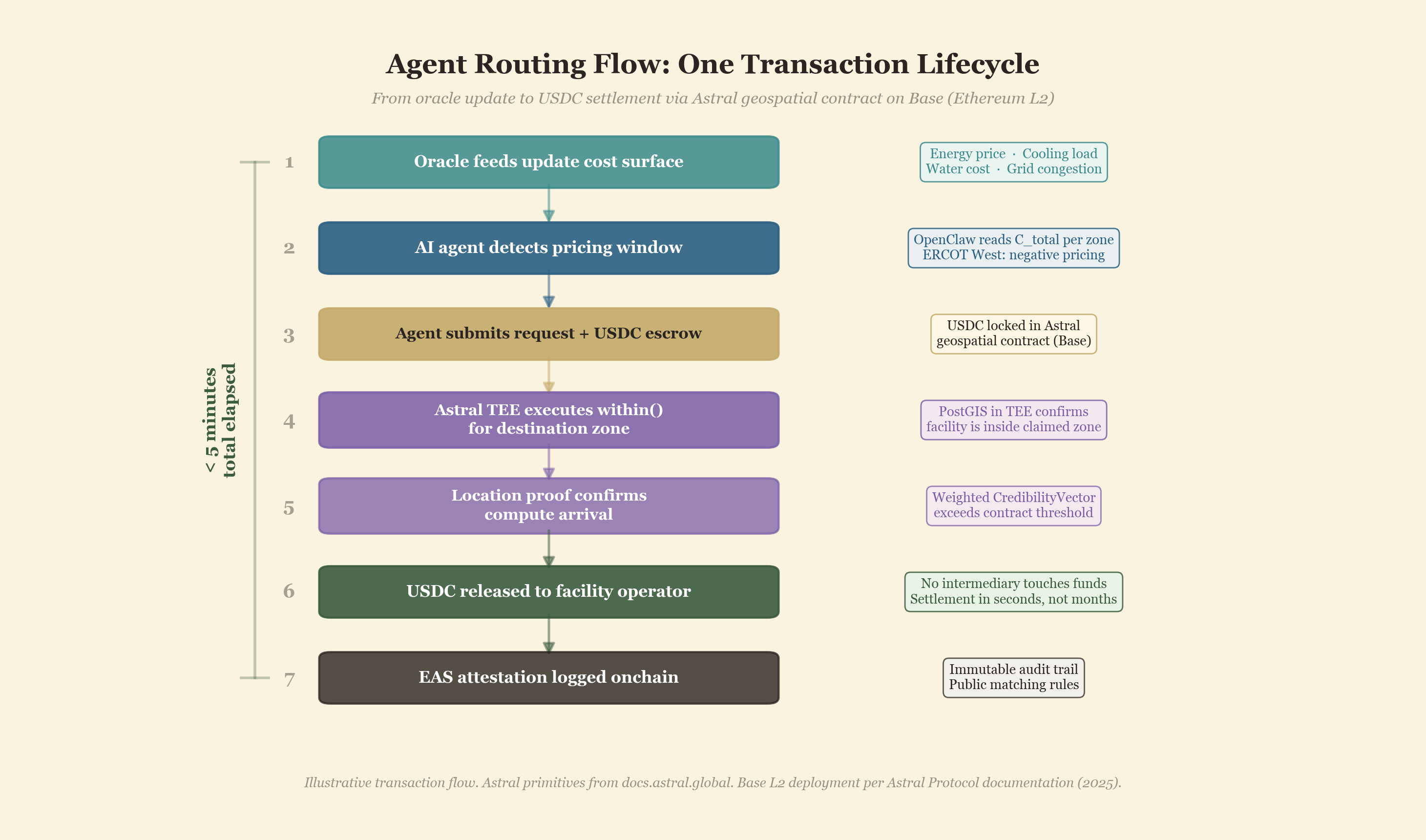
In this case, the topocurrency is not a new token — it is USDC whose settlement is conditioned on spatial verification. The geospatial contract reads oracle feeds, computes C_total per zone, and will not release escrowed funds until a TEE-signed attestation of Astral’s within() result confirms the workload arrived at the claimed location. The spatial query itself executes off-chain in Astral’s Geospatial Policy Engine (PostGIS running inside a TEE); the contract reads the result, verified by the TEE’s signature, not the operation itself. The stablecoin becomes location-aware money not by changing what it is, but by constraining how it moves.

A skeptic observes that Google already routes compute spatially without any cryptocurrency. Why does this mechanism require a token on a public blockchain? The answer is not ideological. It is a claim about four specific market failures that a centralized platform cannot efficiently solve:

1. Transaction costs. Bilateral Power Purchase Agreements take 6–12 months to negotiate and require specialized legal counsel.²⁰ For real-time spatial matching at 5-minute oracle resolution, bilateral contracting is structurally impossible — you cannot renegotiate a PPA every 5 minutes. In financial settlement, smart contracts have already demonstrated the gains from eliminating this friction: JP Morgan’s Quorum platform cut interbank settlement costs by 50–70%, and a controlled study of supply chain contracting found a 76% reduction in per-transaction fees with settlement time compressed by 70%.²¹ Energy markets, where bilateral contracts are even more complex and slower, stand to gain at least as much.

2. Coordination failure. Matching flexible compute demand with spatially distributed renewable supply is a multilateral matching problem.²² Bilateral contracting produces “application waste” and “screening waste”: each negotiation ignores its externalities on all other potential matches. A centralized clearinghouse solves the coordination problem but introduces rent extraction — intermediaries capture a larger share of gains from trade, and intermediation may emerge “exclusively because of rent extraction motives” even when “socially worthless.”²¹ A decentralized clearinghouse (smart contract + oracle) avoids this: the matching rules are public, the execution is automatic, and no single intermediary can extract rent by controlling the matching rules — the rules are the code, visible to all participants.

3. Hold-up. Co-location investments are relationship-specific — once a data center builds next to a wind farm, it is vulnerable to renegotiation. This is the hold-up problem that Oliver Williamson formalized: asset specificity combined with incomplete contracts enables opportunism.²³ Smart contracts function as credible commitment devices — immutable terms, automatic execution — resolving the hold-up without courts or renegotiation.

4. Composability. A centralized spatial matching platform can route compute. What it cannot do is compose the routing with adjacent financial functions in a single transaction. Consider what a facility operator actually needs: not just a matched workload, but insurance against curtailment intermittency (what if the wind dies mid-job?), hedging on energy price movements (what if the cost advantage erodes before the batch completes?), and capital to build the facility in the first place. In traditional markets, each of these requires a separate counterparty, separate collateral, and separate settlement — multiplying transaction costs and locking capital in redundant pools. Onchain, these compose: the same USDC settlement that pays for the routing can collateralize a curtailment insurance position; the onchain revenue history from verified settlements becomes transparent proof-of-income for lending protocols financing new renewable-adjacent facilities; energy price derivatives can be written against the oracle feeds the cost surface already reads. Each function shares the same settlement layer and the same collateral, rather than requiring parallel financial infrastructure.²¹

Global data center electricity consumption is approximately 415 TWh per year.¹⁵ Even applying the 57% cost differential to only the locationally flexible fraction (10–20% of total energy) yields low single-digit billions per year in capturable efficiency gains — before composability benefits.

The honest counterpoint. Centralization is better for high-frequency, low-latency operations where millisecond execution matters. Abadi and Brunnermeier (2018) formalize the blockchain trilemma: a consensus algorithm cannot simultaneously achieve fault-tolerance, resource-efficiency, and full transferability.²⁴ The argument is not that oracle aggregation, route optimization, or workload scheduling must be onchain — these are computation-heavy tasks better handled offchain. It is that the settlement layer and commitment mechanism benefit from decentralization — public rules, automatic execution, and intermediary functions (oracle provision, location verification) that are contestable rather than monopolistic — while the compute routing itself uses offchain optimization that settles onchain.

Le mécanisme en action

The cost differential already exists. In Iceland (100% renewable, PUE 1.05–1.20, ambient cooling year-round), the all-in cost of compute is approximately $45.50/MWh. In Northern Virginia (200–500 gCO2/kWh, PUE 1.4–1.6, mechanical cooling required), it is approximately $106/MWh — energy, cooling, water, and congestion combined.²⁵ The differential is roughly 57%. No rational agent needs to be taxed into choosing the cheaper option. It needs to be shown where the cheaper option is.

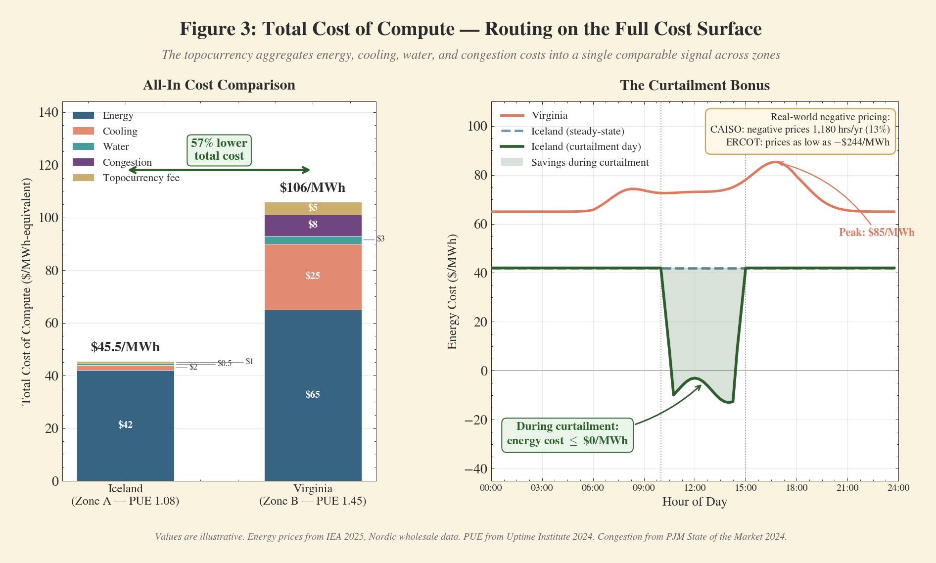
The topocurrency’s job is to make this differential visible and actionable in real time — aggregating energy price, cooling load, water cost, and grid congestion across zones into a single comparable cost surface that any agent can read. The surface has to be real-time because the opportunities are fleeting: a wind ramp in West Texas lasts roughly 45 minutes, ERCOT West Zone prices reached –$244/MWh before reversing within minutes, and CAISO prices were negative for 1,180 hours in 2024 — 13% of all hours.¹³ Bilateral PPAs negotiated over months cannot capture this. An agent reading a live cost surface can.

AI agents — autonomous programs that can read oracle data, evaluate options, and execute transactions — operate at the right timescale. Imagine an agent built on OpenClaw, the open-source framework with over 100,000 installations, configured with a single objective: minimize total cost of compute for a batch training run.²⁶ The agent reads the topocurrency’s cost surface, detects a negative pricing window in ERCOT’s West Zone, evaluates the total cost of migrating a batch training checkpoint to a co-located facility, and executes the move — depositing USDC into the geospatial contract and settling before the window closes. The agent is both the demand (it runs the compute) and the router (it decides where to run it). It is cheaper to move bits than electrons: fiber optic transmission costs approximately $0.25 per terabyte per 1,000 km, while long-distance HVDC electricity transmission exceeds $40/MWh — making compute-at-the-source economically rational whenever the workload tolerates latency.²⁵

The contract the agent settles through is an Astral geospatial smart contract deployed on Base (Ethereum L2). The contract reads oracle feeds for energy price, cooling load, water cost, and congestion at each registered zone, computing C_total per zone on every update. When an agent submits a routing request, it deposits USDC into the contract — locking payment so the facility operator has a guarantee before accepting the workload. Astral’s Geospatial Policy Engine (PostGIS running inside a TEE) then executes the within() query to verify that the destination facility is inside the claimed zone, signing the result as an EAS attestation that the contract can verify. Once the agent’s location proof (carrying a CredibilityAssessment — derived from its CredibilityVector via an application-specific weighting function — above the contract’s threshold) confirms the compute physically arrived, the contract releases the locked USDC to the facility operator and logs the settlement as an EAS attestation onchain. The agent cannot withdraw the deposit without proof of delivery; the operator cannot claim payment without the compute arriving. The intermediation is the contract itself — transparent, auditable, and unable to extract discretionary rent.

At scale, the effect is arbitrage toward equilibrium. Each agent routing a workload to a cheaper zone narrows the cost differential slightly — energy prices rise in the destination as demand increases, and fall at the origin as demand leaves. With hundreds of agents operating on the same cost surface, the differential compresses until marginal routing cost equals marginal savings. The system does not eliminate the differential — geography, climate, and infrastructure ensure persistent cost variation — but it captures the low-hanging fraction.

An estimated 30–50% of AI compute — training, fine-tuning, and batch inference — is temporally deferrable, and for new deployments can in principle be sited at locations with cheaper energy. AI currently represents roughly 14–27% of total data center energy consumption, but its share is growing fastest.¹⁵ The locationally flexible fraction of total data center energy is therefore perhaps 10–20% today — constrained by data gravity (petabyte-scale training sets resist migration), regulatory requirements (GDPR, data sovereignty), and the need for co-located GPU infrastructure at the destination. Even at this smaller fraction, if the average exploitable differential is half the Iceland-Virginia gap, spatial arbitrage represents low single-digit billions of dollars per year in efficiency gains — growing as AI’s share of total compute increases. The effect is geographic redistribution: Iceland’s geothermal advantage, ERCOT West’s curtailed wind, Nordic hydroelectric capacity, Moroccan solar fields, Chilean wind corridors — each becomes a spatial attractor for flexible compute, drawing economic activity toward places with cheap, abundant energy that the grid currently wastes.

The gap between current agent capabilities and this scenario is real but narrow. What the spatial compute market needs is not general-purpose autonomous agents — it needs a specific, bounded capability: read the cost surface, compare zones, and route the next workload batch. The infrastructure is emerging: ERC-8004 (mainnet January 2026) establishes onchain identity and reputation registries for autonomous agents²⁷, and machine-to-machine payment standards (Google’s AP2, x402) provide payment rails.

The formal cost decomposition underlying this mechanism — including the C_total cost surface, illustrative zone parameters, saturation dynamics, and equilibrium limitations — is presented in Appendix A.

Limitations honnêtes

Flexibility is narrower than it looks. The 30–50% “flexible workload” estimate covers training, fine-tuning, and batch inference, but overstates what is practically movable. An ongoing frontier training run — petabytes of data co-located with thousands of GPUs connected by specialized interconnects — cannot be paused and relocated on a 5-minute oracle cycle. Checkpoint transfer for frontier models can consume hours of bandwidth. And routing compute across jurisdictions encounters data sovereignty constraints: GDPR, sectoral privacy regulations, and national security restrictions limit where certain workloads can physically execute, regardless of energy cost. What IS locationally flexible: new training runs not yet started (the siting decision), fine-tuning jobs on public datasets, batch inference with no real-time latency requirement, and synthetic data generation. These are meaningful — but they are a subset of the 30–50%, not the whole of it. The locationally flexible fraction of total data center energy is closer to 10–20% today, as estimated above. The mechanism’s near-term addressable market is the smaller number, growing as AI’s share of total compute increases and as independent GPU providers build capacity at renewable-surplus sites.

The mechanism does not disrupt hyperscalers — it routes around them. AWS, GCP, and Azure control the majority of cloud compute and benefit from hiding spatial cost variation: uniform regional pricing protects high-margin zones, and egress fees ($0.05–0.12/GB, declining with volume) make data gravity a deliberate moat.²⁸ They have no structural incentive to expose a real-time cost surface. But the mechanism does not need them. The AI buildout is driving rapid expansion of independent GPU providers — CoreWeave ($8B projected 2025 revenue), Lambda ($500M+), Crusoe, bare-metal operators — a neocloud market estimated at $24 billion in 2025 and growing over 40% annually.²⁹ These operators compete on price, build at renewable-surplus sites, and have no platform lock-in to protect. The parallel is CDNs: Cloudflare did not replace hosting providers, it created a routing layer on top of them. If hyperscaler adoption comes, it arrives from the demand side — enterprise buyers who need spatial transparency for carbon reporting under the EU’s Corporate Sustainability Reporting Directive (CSRD), which requires Scope 2 emissions disclosure using both location-based and market-based methods³⁰ — not from hyperscaler incentive.

Cost savings first, emissions second. The mechanism optimizes on total cost (energy + cooling + water + congestion), not carbon. The environmental case is therefore derivative: emissions fall only where cheap zones also happen to be clean zones. That overlap is substantial today — Iceland, Nordic hydro, ERCOT wind — but it is not guaranteed. Knittel et al. (2025) demonstrate that flexible data centers reduce emissions only when regional renewable penetration exceeds approximately 50%; below that threshold, load flexibility can support fossil baseload by filling off-peak valleys, increasing emissions.³¹ The topocurrency must target geographies above this threshold or risk the paradox of flexibility enabling fossil generation. A zone that is cheap because of lax environmental regulation, not renewable abundance, would attract compute under this mechanism just as effectively — the cost surface is agnostic about why a zone is cheap. And at the macro level, making clean-zone compute cheaper may accelerate total compute demand (Google’s emissions rose 50% despite carbon-aware computing) — the mechanism routes demand more efficiently, not less of it.

The model assumes a static cost surface; reality won’t be. The formalization in Appendix A asks: given a cost surface, how does a single agent respond? It does not model what happens when thousands of agents respond simultaneously — and their collective behavior changes the surface itself. If flexible compute floods Iceland, land prices rise, labor gets scarce, and grid congestion appears where there was none. The cost advantage that attracted the compute erodes because the compute arrived. Conversely, agglomeration economies (shared infrastructure, specialized labor pools) could make popular destinations cheaper over time, concentrating activity further. Which effect dominates is an empirical question that requires spatial general equilibrium modeling — the framework Balboni and Shapiro (2025) identify as the frontier for this kind of analysis.³² The formalization here does not attempt it. The surface also shifts from the supply side: battery storage deployment is reducing curtailment — CAISO alone added 3.6 GW of battery capacity in 2024 — and grid expansion eventually reaches remote generation sites.¹³ A compute facility built on the assumption of permanently cheap curtailed energy may find its cost advantage eroding as infrastructure catches up. The topocurrency’s oracle-driven pricing mitigates this dynamically: as curtailment falls and prices normalize in a zone, the cost advantage diminishes automatically and workloads route elsewhere. But physical infrastructure cannot move.

Curtailment alone is not enough. The mechanism’s most vivid price signal — negatively priced curtailed energy — is a finite resource. Global curtailment in 2024 was approximately 100 TWh.¹³ The locationally flexible fraction of data center energy — roughly 10–20% of 415 TWh, or 40–80 TWh¹⁵ — is meaningful relative to curtailment, but curtailed energy is geographically concentrated and temporally intermittent. The topocurrency must therefore route to all cheap-renewable zones, not just curtailed ones; curtailment is the sharpest signal, not the only one.

Oracle reliability, location spoofing, and fee-gaming risks that apply across all topocurrency mechanisms — including spatial compute — are addressed in What Stands in the Way.

---

L'espace de conception des topocurrencies

The spatial compute case went deep on one mechanism — a matching platform that routes flexible workloads toward the lowest total cost. But the underlying architecture — geospatial smart contracts that modify economic behavior based on verified location — supports a wider set of mechanisms — fee modulation to price externalities, service-backed minting to reward verified ecological work, and spatial yield distribution to channel value through landscapes, among others. Each addresses a different failure in the relationship between money and geography.

Every territory has capital that markets currently cannot see. Drawing on the capitals framework from sustainability accounting and community development literature,³³ six categories determine a territory’s capacity: natural capital (ecosystem services), energy balance (renewable fraction, grid carbon intensity), material flows (extraction rates, circular economy metrics), institutional capital (governance density, rule-of-law indicators), social capital (trust networks, associational density), and infrastructure topology (transport, digital connectivity, utilities). Today, a territory’s credit rating depends on tax revenue and debt levels, not on whether its aquifers are depleting or its social fabric is intact. Topocurrencies make this fiscal profile legible and investable — legible because the oracle infrastructure required to price transactions (grid carbon intensity, water stress indices, land use data, biodiversity metrics) forces territorial capital into a standardized, real-time, machine-readable format; investable because a staking position in a zone contract converts that data into yield, with returns proportional to ecological quality multiplied by transaction volume.

Conventional banking makes the problem worse. Sheila Dow demonstrated that regional financial markets are segmented by portfolio preference; Chick and Dow showed that banking consolidation systematically moves liquidity from periphery to core.³⁴ The New Economics Foundation’s LM3 metric quantifies the effect: every pound spent locally generates £1.76 in local activity, versus 36 pence spent outside — a fivefold difference.³⁵ A Kenya RCT found that blockchain-based community tokens achieved a 3.1x local multiplier.³⁶ The Swiss WIR Bank — operating since 1934 among 60,000+ member businesses — demonstrates that the pattern holds over nine decades.³⁷

The topocurrency mechanism is geographic containment: with contains() gating, tokens circulate within a territory’s boundary rather than leaking to external markets, creating a local recirculation loop that conventional banking structurally lacks.

The result is an investable instrument. A staking position in a zone contract earns returns funded by fee differentials between zones — not by external subsidy or token inflation. Unlike green bonds, which are evaluated by annual audits and priced on issuer credit, topocurrency yields respond to real-time oracle data at zone-level granularity. The feedback loop is direct: improve conditions → increase reward rate → attract capital → fund further improvement — a “territorial yield curve” indexed to ecological health rather than sovereign creditworthiness.

Deux architectures de jetons

Before mapping those mechanisms, a foundational choice: where does the token come from? Two primary architectures exist — one takes a global asset and localizes it, the other incubates a new local asset — and the choice determines the token’s economic properties, sovereignty, regulatory exposure, and institutional requirements.

Path A: Stablecoin Capture. A user deposits USDC (or another established stablecoin) into a geospatial smart contract. The contract applies spatially-varying rules based on oracle data, but no new monetary supply is created — the topocurrency layer modulates transaction costs and incentives, not the underlying money. Modern stablecoins generate yield from reserve assets (Circle’s USDC earns Treasury-bill returns³⁸), and a geospatial contract can capture this yield and redistribute it spatially. This is the pragmatic choice: it inherits stablecoin liquidity from day one, leverages proven DeFi infrastructure, and avoids the cold-start problem of building a new currency. The cost is dependency on the stablecoin issuer’s regulatory and counterparty risks.

Path B: Service-Backed Minting. Verified outcomes at a verified location trigger new tokens — mangrove hectares restored, watershed health maintained, sensor networks deployed, local commerce sustained. Which outcomes qualify is a governance decision: the territory sets mint_rate and burn_rate, controls its own monetary policy, and backs the currency with its own productive capacity. This is the sovereign choice. The cost is bootstrapping — though once adoption crosses a critical threshold, local multiplier effects can be substantial. Mutual credit networks — WIR Bank in Switzerland, Sardex in Sardinia³⁷ — are historical precedents; Path B extends their logic with verifiable outcomes, programmable rules, and composability with global finance.

Table 2: Two token architectures for topocurrencies.

	Path A: Stablecoin Capture	Path B: Service-Backed Minting
Token origin	External stablecoin deposited into geospatial contract	New token minted upon verified spatial outcome
Monetary supply	Fixed — no new money created	Expands with verified work
Liquidity	Inherits stablecoin liquidity from day one	Must build own liquidity through adoption
Sovereignty	Depends on external issuer (Circle, Tether)	Territory controls monetary policy
Bootstrap difficulty	Low — DeFi escrow/AMM infra exists	High — needs local adoption loop
Yield source	Baseline stablecoin yield (T-bill reserves) + spatial rewards	Territorial revenue sharing only — no exogenous yield floor
Best for	Carbon/compute, tourism, humanitarian, supply chain	Bioregional ecology, cultural sovereignty, watershed

These two cover the primary design space, but they are not exhaustive. Hybrids are possible — e.g., partial stablecoin collateral plus partial service-backing.

Mécanismes et flux spatiaux

A topocurrency needs two things: a mechanism — the rule that determines how tokens behave — and a spatial flow — the pattern by which value moves through geography. The mechanism is the economic logic; the spatial flow is the geographic logic. Together they define what a topocurrency does and where it does it. A third dimension — the institutional anchor — determines who provides legitimacy and enforcement: an energy oracle, a community governance body, a municipal authority, a humanitarian agency. No mechanism works without one.

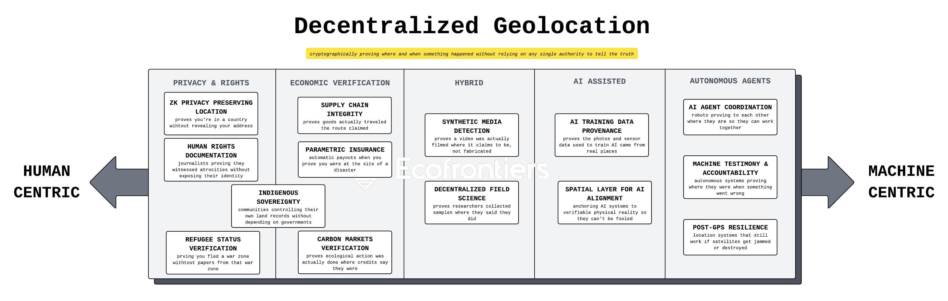
Eight mechanisms. The design space includes eight distinct mechanisms:

1. Geospatial fee modulation — same token, different costs by location. Fees and rewards shift based on real-time spatial data from oracles. (Carbon pricing, externality internalization.)
2. Stablecoin capture — existing stablecoins locked into geospatial contracts that constrain where they circulate, keeping external liquidity recirculating locally. (Tourism, humanitarian aid.)
3. Service-backed minting — new tokens created when verified outcomes occur at a verified location, expanding monetary supply in proportion to measurable results. (Bioregional ecology.)
4. Spatial yield distribution — yield distributed based on where holders are, not just how much they hold. Geography determines who benefits from returns. (Watershed services.)
5. Location-contingent vesting — tokens unlock only with sustained verified presence over time. Rewards commitment to a place, not transient visits. (Bioregional sovereignty variant, supply chain provenance.)
6. Territorial revenue sharing — a percentage of economic activity within a geofenced zone is automatically redistributed to local stakeholders. Programmable local taxation. (Infrastructure, bioregional governance.)
7. Spatial matching — a two-sided platform connecting geographically flexible demand with locationally fixed supply, routing activity toward the lowest total-cost sites. Unlike fee modulation (which taxes externalities), spatial matching works because the destination is already cheaper. (Spatial compute, flexible load balancing.)
8. Spatial bonding curves — token price is a function of geographic demand. Cheaper in underserved areas, more expensive in saturated ones. (Compute siting, service provision in underserved regions.)

These mechanisms can combine. A bioregional ecology contract might use service-backed minting (3) for issuance, territorial revenue sharing (6) for redistribution, and spatial yield distribution (4) to channel endowment returns to verified stewards.

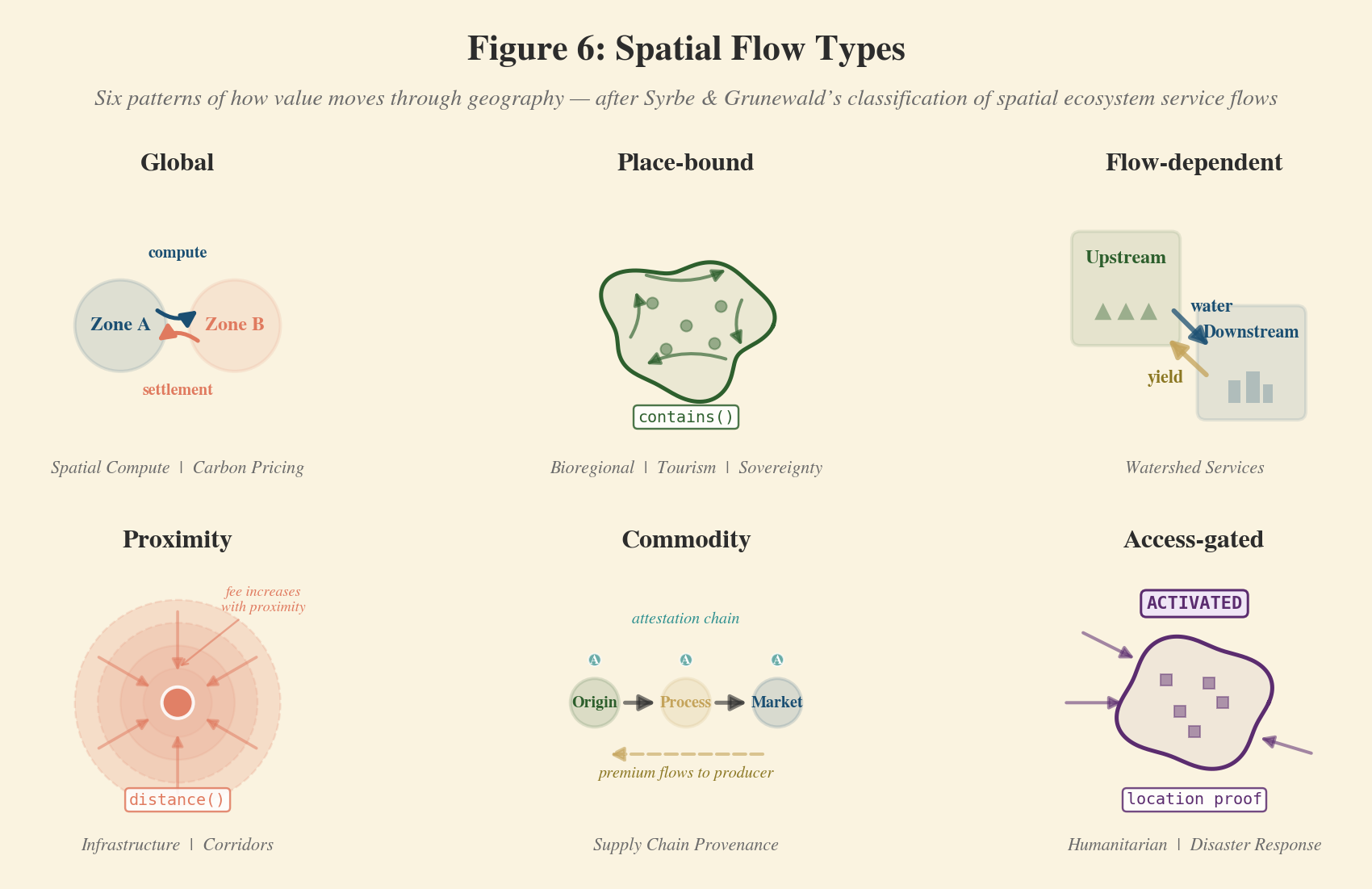
Six spatial flows. Each use case also has a characteristic spatial flow — the pattern by which value moves through geography.³⁹

• Global — value flows anywhere; no geographic constraint on where benefit accrues. Compute routes globally; carbon credits trade globally.
• Place-bound — value circulates within a territory. A bioregional currency stays in the bioregion; tourism revenue stays in the destination.
• Flow-dependent — value follows a physical path: water, nutrients, air. Downstream economic beneficiaries fund upstream stewards.
• Commodity — value travels with a physical good from origin to destination. Provenance attestations move with the product.
• Proximity — value decays with distance from a corridor or point of infrastructure. Benefits concentrate near the asset.
• Access-gated — value is available only to verified participants within a zone. Humanitarian aid reaches verified recipients, not intermediaries.

The table below maps each use case to its primary mechanism, spatial flow, institutional anchor, and the Astral geospatial primitive — within(), contains(), distance() — that implements the spatial logic. These primitives execute off-chain in Astral’s Geospatial Policy Engine (PostGIS in a TEE); contracts read the TEE-attested results, not the operations themselves.⁷

Table 3: Eight use cases mapped to mechanism, spatial flow, and institutional anchor.

Use Case	Primary Mechanism	Spatial Flow	Astral Primitive	Institutional Anchor
Spatial compute	Spatial matching + fee modulation	Global	within()	Energy/environmental oracles
Carbon pricing	Fee modulation	Global	within()	Carbon registries (EU ETS, VCMs)
Bioregional ecology	Service-backed minting + revenue sharing	Place-bound	contains()	Community governance, MRV oracles
Watershed services	Spatial yield distribution	Flow-dependent	within()	Cross-jurisdictional water compact
Tourism / destinations	Stablecoin capture	Place-bound	contains()	Destination management org
Supply chain provenance	Location-contingent vesting	Commodity	Origin attestation	Producer cooperatives
Infrastructure / corridors	Revenue sharing + fee modulation	Proximity	distance()	Municipal authority
Humanitarian / disaster	Stablecoin capture	Access-gated	Location proof	Humanitarian agencies

Spatial Compute

Mechanism: spatial matching + fee modulation. Components deployed. Formalized in Appendix A. The topocurrency operates as a two-sided matching platform on existing stablecoins, connecting locationally flexible compute demand with stranded or underutilized renewable supply. The primary value proposition is total cost — energy, cooling, water, congestion — not the topocurrency fee, which sharpens an economic gradient that already exists. No new token is minted. Deployed precedents include Google’s carbon-intelligent computing¹⁶, Crusoe Energy’s stranded-asset compute, and Riot Platforms’ grid-interactive mining in ERCOT.¹⁹

Carbon Pricing

Mechanism: geospatial fee modulation. Theoretical. Where spatial compute routes activity toward low-cost locations, carbon pricing applies the Pigouvian logic directly: make externalities visible at the point of transaction, and let the fee gradient do the work. Existing carbon registries — EU ETS (€781 billion traded in 2024), Article 6 mechanisms, voluntary markets ($535 million) — price carbon uniformly within broad jurisdictions.⁴⁰ Montgomery (1972) proved this is suboptimal: marginal damages and abatement costs vary by location, and spatially differentiated pricing captures welfare gains that uniform pricing leaves on the table.⁴¹

Tokenizing registry issuances unlocks benefits that the current infrastructure cannot provide. EU ETS allowances currently clear through national registries with multi-day settlement and opaque transaction records; tokenized allowances settle atomically, with every issuance, transfer, and retirement publicly verifiable onchain — eliminating the counterparty risk and double-counting that plague both compliance and voluntary markets. Tokenized allowances become composable: usable as collateral in DeFi lending markets, bundable into structured environmental products, and integratable into automated compliance workflows that retire allowances at the point of emission rather than through annual reconciliation. Standardized token interfaces could link registries across jurisdictions — EU ETS, California cap-and-trade, Korea ETS — achieving the cross-border interoperability that Article 6 envisions but no bilateral agreement has delivered.

A topocurrency adds a spatial layer on top of these tokenization benefits. An EU ETS allowance currently trades identically whether it retires a ton of CO₂ from a lignite plant in Silesia or a gas turbine in the Netherlands — yet the co-pollutant damages at those two locations differ by an order of magnitude. A topocurrency fee layer indexed to real-time spatial data — grid carbon intensity (via WattTime or Electricity Maps), water stress (WRI Aqueduct), and land use — adds the geographic dimension that the registry itself lacks. Transactions in carbon-intensive zones pay higher fees; that fee revenue funds rewards in low-carbon zones. The registry handles the carbon accounting; the tokenization handles the settlement and composability; the topocurrency handles the spatial pricing. Location metadata travels with the instrument from issuance through every transfer to retirement.

A Pigouvian tax sets the price of an activity equal to the damage it causes — the polluter pays the social cost, not just the private cost. The case for spatial differentiation is strongest where the uniform price is most wrong, and carbon markets get this wrong in a specific way. CO₂ itself is a uniformly mixed pollutant: a ton emitted in Silesia and a ton emitted in Rotterdam cause identical climate damage, so a uniform carbon price is defensible for CO₂ alone. But burning fossil fuels doesn’t just release CO₂. The co-pollutants — PM2.5, SO₂, NOₓ — cause health damages that vary dramatically by location: a ton of coal burned upwind of a dense population center causes far more respiratory illness, cardiovascular disease, and premature death than the same ton burned in a sparsely populated region. No existing carbon registry prices this difference.

The welfare cost of ignoring spatial variation is large. Hollingsworth et al. (2022) estimate that the failure to spatially differentiate U.S. air quality regulation alone costs $70 billion per year in foregone welfare — health damages that could be avoided if pollution prices reflected where the pollution actually lands.⁴² A tokenized spatial layer on the EU ETS could yield €3–6 billion per year in combined efficiency gains: settlement cost elimination from onchain clearing, capital efficiency from composable allowances, and spatial differentiation of co-pollutant damages.⁴²

Bioregional Ecology

Mechanism: service-backed minting + territorial revenue sharing. Piloted. The global payment-for-ecosystem-services (PES) market exceeds $36 billion annually across 550+ programs, with watershed services the largest sector at $24.7 billion.⁴³ Yet less than 1% of global climate finance reaches local communities directly — intermediaries absorb the rest. Unlike the spatial compute and carbon pricing cases, which modulate fees on existing stablecoins, bioregional ecology creates new money — tokens minted when verified ecological work happens at verified locations.

Consider the Galapagos Marine Corridor (CMAR), where Costa Rica, Panama, Colombia, and Ecuador share jurisdiction over a continuous marine ecosystem.⁴⁴ Here, the topocurrency creates new money — tokens minted when MRV oracles verify restoration work and location proofs confirm presence. This is fundamentally different from stablecoin capture: the monetary supply expands in proportion to verified ecological stewardship, and the contains() primitive enforces the bioregional boundary — driving the liquidity retention effects described above.

The same mechanism extends to local economic sovereignty — communities in resource-rich peripheral regions where extraction revenues flow outward while local populations bear environmental and social costs. U.S. tribal lands alone contain 50% of potential uranium reserves and 20% of known oil and gas reserves, with extraction value flowing predominantly to external operators. Because the token is minted through verified local activity — not purchased on an exchange — participation in the territory’s economic life is the only way in.

Watershed Services

Mechanism: spatial yield distribution. Theoretical — inspired by deployed PES programs. Watersheds create a natural upstream-downstream dependency: forests and wetlands upstream filter water, regulate flow, and prevent erosion — services that downstream cities and farms consume but rarely pay for. The economic logic of paying upstream stewards is well established. New York City’s Catskills watershed protection program cost $1.5 billion over a decade; the alternative — a filtration plant — was estimated at $6–10 billion to construct plus $1 million per day to operate, a 4–7x cost ratio.⁴⁵ But existing payment-for-ecosystem-services (PES) programs run on bilateral contracts and grant cycles — intermittent funding tied to political budgets rather than continuous compensation proportional to outcomes.

A topocurrency makes the payment continuous and spatially precise. The funding source is the downstream beneficiary: a water utility allocates a fraction of its ratepayer revenue into a smart contract, or a conservation trust locks capital into a yield-bearing position and directs the returns upstream. Either way, the money flows from those who consume the service to those who produce it — automatically, without grant applications or bilateral negotiation. Distribution is weighted by verified spatial location within the watershed’s flow corridor: the TEE-attested result of the within() primitive confirms that stewardship occurs in the hydrologically relevant zone, and water quality metrics from IoT sensors determine how much yield each steward receives. Stewards who maintain forest cover in high-impact catchment areas earn more than those in low-impact zones — the yield reflects the spatial value of the service, not just the area of land maintained. The spatial flow is directional: water flows downstream, yield flows upstream.

Tourism / Destination Economies

Mechanism: stablecoin capture. Theoretical. Tourism is one of the most spatially leaky industries. UNCTAD estimates 40–50% import-related leakage of gross tourism earnings for small economies; in least-developed destinations, the figure reaches 80%.⁴⁶ A tourist pays $200 for a hotel night in Bali, but most of that leaves immediately — to the international chain’s headquarters, to imported food suppliers, to foreign booking platforms. The local economy sees a fraction of the spending that physically occurs within its borders.

The topocurrency’s job is to capture the foreign currency permanently. When a visitor converts stablecoins into a geospatially-constrained token via contains() gating, that money enters local circulation and stays there. Local merchants, guides, and service providers transact in the constrained token. When they spend it at other local businesses, it recirculates — each transaction multiplying its local impact rather than leaking to external operators. The stablecoin backing remains locked in the contract as a reserve, but the local token circulates indefinitely within the territory, functioning as captured foreign exchange. The more tourists spend, the larger the local monetary base, and the more the territory can invest in the amenities that attract further visitors.

Supply Chain Provenance

Mechanism: location-contingent vesting. Theoretical. The global fair trade market exceeded $12 billion by 2021 and continues to grow. Organic certification fraud costs legitimate U.S. producers hundreds of millions of dollars — a consequence of paper-based auditing that occurs at discrete intervals rather than continuously.⁴⁷ A stablecoin escrow is linked to goods at their production origin via location-verified attestation. The escrow vests — releases payment to the producer — only when location proofs confirm the goods were produced at the claimed origin and downstream quality checks pass. Provenance metadata is embedded cryptographically: where the coffee was grown, where the mineral was extracted, where the garment was sewn. Downstream buyers pay a premium for verified-origin goods; the premium flows to producers through the vesting contract. This replaces trust-based certification (Fair Trade, conflict-free minerals) with cryptographic spatial verification — and unlike paper audits, the verification is continuous and tamper-evident.

Infrastructure / Corridor Funding

Mechanism: territorial revenue sharing + geospatial fee modulation. Theoretical. McKinsey estimates the global infrastructure investment gap at $350 billion per year — $3.7 trillion needed annually through 2035 against current spending. Municipal bond issuance costs average 1% of principal, imposing $4 billion annually in intermediary fees across 13 categories of service providers in the U.S. alone.⁴⁸ Transport corridors, water networks, and broadband infrastructure serve spatially-defined user populations. The topocurrency collects fees from users within the corridor — modulated by distance() from the infrastructure, so heavier users closer to the asset pay more — and allocates collected fees to maintenance and expansion. The closest deployed analogue is congestion pricing: London’s congestion charge and Singapore’s ERP system both modulate fees by location and time to manage infrastructure demand, though neither is programmable or composable with other financial instruments. A spatial bonding curve could extend the idea further: the token price becomes a function of geographic demand — cheaper in underserved areas, more expensive in saturated ones — so that high demand algorithmically generates the revenue to build more capacity.

Humanitarian / Disaster Response

Mechanism: stablecoin capture. Deployed. The World Food Programme’s Building Blocks blockchain has processed $555 million in cash-based transfers, saving $3.5 million in bank fees and preventing $287 million in aid duplication across 65 organizations in Ukraine alone — a 98% reduction in transaction costs, serving 4 million people per month.⁴⁹ Donor-funded stablecoins are locked into geospatial contracts that activate only in designated crisis zones. Location proofs with high CredibilityAssessment thresholds (derived from CredibilityVector weighting tuned for humanitarian contexts) ensure aid reaches people physically present in the affected area. The contract prevents diversion — funds cannot be spent outside the crisis boundary — and provides real-time transparency to donors on where and how aid flows. When the crisis designation lifts, remaining funds can be released or redirected. This is the clearest case for pure stablecoin capture: the backing is the donated USDC itself, the geography is the crisis zone, and the constraint is what prevents the aid from being stolen.

---

Ce qui se met en travers

Topocurrencies are not inevitable. The challenges are technical, institutional, and economic — and the AI Institutional Design Atlas provides a framework for assessing them.¹⁴

Défis techniques

Location spoofing at scale. Location proofs raise the cost of lying, but they don’t eliminate it. A well-resourced actor could theoretically compromise multiple stamp sources simultaneously. Astral’s framework acknowledges this directly: GPS is spoofable, which is why verification produces a multidimensional CredibilityVector rather than a binary gate — the vector captures independent dimensions of evidence quality, and applications set thresholds on a weighted CredibilityAssessment derived from it. The defense is multi-signal composition and the economic principle established earlier — that forgery cost must exceed transaction value — but the arms race between provers and spoofers will be ongoing.

Oracle reliability. Topocurrencies that respond to real-world data are only as good as that data. Energy price feeds lag or report stale values. Satellite imagery has gaps. IoT sensors fail. Compromised oracles cause contracts to execute on false information — not merely inaccurate but credibility-destroying. The oracle industry is converging on defense-in-depth: multi-source aggregation prevents any single provider from corrupting a feed; economic staking slashes operator collateral for provably incorrect reports; freshness requirements reject stale data; TWAP smooths transient anomalies; and circuit breakers halt execution when values deviate beyond thresholds — patterns battle-tested in DeFi protocols managing billions in collateral. For topocurrencies, the defense extends further: energy feeds cross-reference multiple ISOs, satellite data validates against ground-truth sensors, and location proofs already use multi-signal composition (GPS, WiFi, cell tower, IP) because no single source is trustworthy alone. The residual risk is correlated failure — multiple independent sources simultaneously wrong — which is real but diminishing as data source diversity increases.

Sybil attacks on spatial rewards. Location proofs address where, but not who. If a topocurrency rewards presence at a location, what prevents a single actor from creating multiple identities to claim multiple rewards at the same coordinates? The intersection of spatial verification and identity verification (proof-of-personhood) is a fundamental design challenge that no current system fully solves.

Data integrity incentives. If a topocurrency’s value rises when its underlying indicators improve — ecological health, energy surplus, provenance verification, local transaction volume — the incentive to fabricate improvement data is significant. Robust topocurrencies need adversarial separation between data production and economic benefit — those who profit from the data cannot also be those who produce it without independent verification.

Défis institutionnels

Governance capture. Who draws the boundaries of a topocurrency zone? Who decides which oracle feeds matter — and how they’re weighted? Who sets the fee schedule, the minting thresholds, the reward distribution? These are political questions with economic consequences, whether the zone is a bioregion, a grid operator’s territory, a tourism destination, or a humanitarian corridor.

Democratic deficit. Automated systems making allocation decisions that are functionally political — which zone gets fee relief? which watershed gets restoration funding? which community receives emergency resources? where does the next compute facility route? — without democratic accountability. The graduated autonomy pattern — human checkpoints on allocation decisions above a threshold — introduces its own failure mode: escalation flooding, where override requests overwhelm human oversight capacity, degrading the system to rubber-stamping.

Enclosure. A dominant actor forking an open protocol proprietary, locking in users, and extracting rent from the data commons. Data produced with topocurrency incentives must be open commons by construction. Polycentric governance — Elinor Ostrom’s framework for managing commons through nested, overlapping institutions rather than centralized authority — offers the best available template, but implementation remains hard.⁵⁰

Mechanism-specific vulnerabilities. Each topocurrency mechanism introduces distinct failure modes beyond the general categories above. Spatial yield distribution is vulnerable to yield allocation gaming — falsifying location to claim returns intended for a different zone, a principal-agent problem where downstream beneficiaries who control the yield pool have incentives to minimize payouts to upstream stewards. Location-contingent vesting requires careful threshold calibration: too low enables brief-presence gaming (meeting the letter of the rule without the spirit), too high excludes legitimate seasonal or nomadic participants. Spatial bonding curves are susceptible to coordinated price manipulation — agents buying in underserved areas to inflate the price, then dumping on later entrants. And territorial revenue sharing faces a boundary definition problem: who qualifies as a local stakeholder? Too broad and the revenue share dilutes into meaninglessness; too narrow and it excludes legitimate claimants.

Défis économiques

Fee-gaming. Agents register in low-fee zones while operating elsewhere — claiming a “clean” grid location for compute, a protected-area address for carbon credits, or a local residency for tourism revenue sharing. Location proofs exist to address this, but the defense requires that activity carry verifiable location attestations with a CredibilityAssessment threshold high enough to make spoofing uneconomic. The deeper problem is Goodhart’s Law applied to spatial pricing: once agents understand the fee adjustment function, they optimize against it.¹⁴

Commons depletion. A low-cost zone attracts so much activity that it exhausts the surplus that made it cheap — a renewable region’s energy advantage disappears under load, a tourist destination’s appeal degrades under overcrowding, a watershed’s capacity is consumed by the upstream activity it incentivized. The saturation constraint r(z,t) → 0 as utilization(z,t) → capacity(z) is the formal mitigation — but calibrating the constraint requires accurate capacity data that may itself be gameable.

Information asymmetry. Agents with faster access to oracle data gain systematic advantages over other participants. In spatial compute, agents with private grid data front-run cost surface changes. In carbon pricing, traders with better emissions models dominate credit markets. In supply chain provenance, large buyers with proprietary logistics data extract better terms. The mitigation — publicly queryable oracle feeds — is necessary but may be insufficient against well-resourced actors who process public data faster than others can.

Leakage and adverse selection. The worst actors simply avoid the system. In environmental economics this is called “leakage”: regulation in some jurisdictions drives dirty activities to unregulated ones.³² The pattern generalizes: compute operators who don’t want spatial transparency route through non-participating platforms; supply chains with something to hide avoid provenance tracking; tourism operators who extract value skip the local currency. A topocurrency that only the already-virtuous participate in concentrates improvement within its boundaries while displaced harm continues outside them. This may ultimately require buyer mandates, regulatory integration, or border adjustment–style mechanisms to address.

Markets already price geography. If a neighborhood has clean air, good water, and low flood risk, rents are higher. This is not a hypothesis — Jennifer Roback formalized it in 1982: environmental amenities are capitalized into land values and wages through spatial equilibrium.⁵¹ The implication is uncomfortable. If markets already encode environmental quality into prices, a topocurrency that does the same thing looks redundant. The signal already exists; it lives in the housing market. The deepest gap is directionality: Roback capitalization rewards living in nice places but does not reward making places nicer. High rents compensate the landowner, not the upstream watershed manager whose conservation keeps the air clean. A topocurrency that ties issuance to verified ecosystem service provision creates a direct incentive for ecological improvement — not just a premium for existing quality. Two further gaps matter. Legibility: housing markets bundle environmental quality into aggregate rent alongside school districts, commute times, and neighborhood prestige — the ecological signal is entangled and invisible as a distinct factor. The oracle infrastructure a topocurrency requires — carbon intensity feeds, water stress indices, biodiversity metrics — forces ecological value into explicit, decomposed, machine-readable format as a necessary byproduct. Speed: housing markets adjust over months to years; topocurrency pricing updates at oracle cadence. This advantage is strongest for rapidly-shifting variables like energy prices and grid congestion, and weakest for slow-moving amenities like air quality or flood risk, where Roback capitalization may keep pace.

Data bootstrapping fragility. Data layer constraints — siloed repositories, high collection costs, coverage gaps — are most acute in precisely the places that need topocurrencies most: remote bioregions with sparse monitoring, developing-country energy grids with unreliable price reporting, informal tourism economies with no transaction data.⁵² A topocurrency can create a virtuous cycle: the currency rewards data production (monitoring, sensor deployment, transaction logging), the data improves the currency’s accuracy (better signals mean better-calibrated issuance and fees), and improved accuracy attracts investment (investors can trust the fiscal profile). But this virtuous cycle is also a fragility. If the cycle breaks — data gets enclosed by early participants, infrastructure degrades without maintenance funding, or a currency loses credibility before the data layer reaches critical mass — the whole system collapses. The bootstrapping problem is severe: a topocurrency needs good data to be credible, but generating good data needs the economic incentives the currency provides. This requires that data produced with topocurrency incentives remain open commons by construction, and that initial data infrastructure be funded through mechanisms (grants, philanthropic capital, government investment) that do not depend on the currency’s own success.

---

La carte devient le territoire

A dollar earned by destroying an old-growth forest is identical to a dollar earned by restoring one — the abstraction compresses away all spatial reality. Topocurrencies introduce financial abstractions that preserve geographic information rather than erasing it. A topocurrency earned by restoring a watershed carries the watershed’s coordinates, the ecological data that verified the restoration, and the location proofs that confirmed presence. The money remembers where it came from.

Eight use cases — from spatial compute routing to carbon pricing to humanitarian aid — demonstrate the same underlying primitives: location proofs, geospatial smart contracts, and environmental oracles, composed into mechanisms ranging from fee modulation to service-backed minting to spatial yield distribution, each converting latent territorial assets into active economic instruments. Most resist the liquidity drift that conventional banking imposes — retaining value within the territory that generates it, or redistributing it toward the places that produce the ecological and social outcomes everyone else depends on.

In a world where AI agents increasingly manage economic activity — allocating capital, evaluating projects, executing transactions — whether those agents understand geography becomes a design question with structural consequences. An AI agent operating in an economy of topocurrencies cannot ignore the physical world, because the economic rules encode it.

The challenges are real. But consider what the pieces assemble into.

Aller plus loin : la surface liée

The bonded surface is the general theory underlying all topocurrency mechanisms — the object that determines how ecological price signals evolve in response to activity. Every mechanism in this essay composes with it differently: spatial compute routes on total cost, of which the ecological price is one component; carbon pricing modulates fees directly on the ecological price; bioregional minting rates respond to it. The surface itself is one object.

Every transaction on the bonded surface pays a fee determined by its location on a planetary pricing map. Transactions in ecologically costly locations — fossil-heavy grids, water-stressed regions, degraded land — pay higher fees. That fee revenue funds rewards in ecologically efficient locations. As activity concentrates in a cheap zone, its ecological surplus gets consumed: energy demand rises, water tables draw down, land use intensifies. The local price rises in response, and activity redistributes to the next cheapest zone. No central authority directs the flow — the price gradient does the work, and the surface self-adjusts.

The eight use cases above operate at bioregional or corridor scale. But the underlying mathematical object has no intrinsic scale limit. Where the case studies work with discrete zones — C_total(z,t) for spatial compute, P_eco(z,t) for carbon pricing — the bonded surface generalizes to continuous coordinates:

P(lat, lon, t) = Σᵢ wᵢ · Cᵢ(lat, lon, t)

A continuous function P: S² → ℝ⁺ assigns a price modifier to every point on Earth’s surface — a scalar field on the sphere, like temperature or barometric pressure, but encoding the ecological cost of economic activity at each location. The data layers to populate it already exist at planetary resolution: grid carbon intensity, water stress, biodiversity indices, soil health, land cover, air quality, and ocean health.⁵³ Stack them with governance-set weights and you have a Locational Marginal Ecological Price — continuous across the planet rather than discretized into zones.

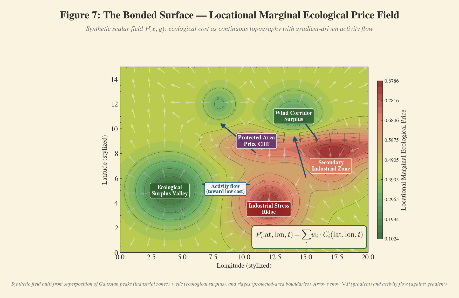
Now add the bonding curve: the surface responds to activity. As economic activity concentrates at a location, the price there rises — because the influx consumes the ecological surplus that made it cheap. Activity flows along gradients toward low-cost regions, the gradients respond to activity, and the system seeks dynamic equilibrium. Ecological load curves economic-space the way mass curves spacetime — activity follows paths of least cost, but activity itself changes the curvature. And the curvature is not uniform: watershed boundaries, mountain ranges, and atmospheric transport patterns create path dependencies. A CO₂ molecule emitted in Shanghai affects Miami differently than one emitted in São Paulo.

To make the dynamic concrete, consider three zones over two time steps:

Table 4: Bonded surface dynamics — three zones over two time steps.

	Zone A (Iceland)	Zone B (West Texas)	Zone C (Virginia)
t=0: P_eco	0.05	0.35	0.72
t=0: C_total	$45/MWh	$58/MWh	$106/MWh
Compute inflow	High	Medium	Low
t=1: P_eco	0.12 (↑)	0.30 (↓)	0.72 (→)
t=1: C_total	$52/MWh (↑)	$54/MWh (↓)	$106/MWh (→)

As compute concentrates in Zone A, its ecological surplus is consumed — energy demand rises, PUE increases with density, and C_total rises. The saturation constraint kicks in: rewards decline, and the next marginal workload routes to Zone B instead, where curtailed wind is being absorbed and local costs fall as the energy finds a buyer. Zone C remains expensive because its grid congestion, cooling costs, and carbon intensity have not improved. The surface self-adjusts without central direction. The resolution need not be uniform: coarse over open ocean (100km), medium over rural land (10km), fine over cities (100m), hyper-fine over contested ecological zones (10m) — higher curvature where the ecological stakes are higher.

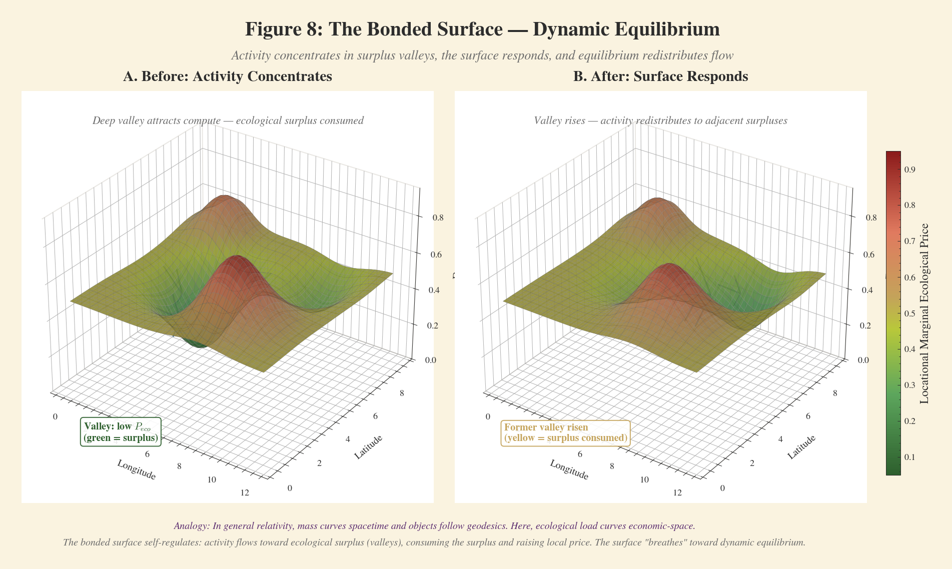
This is what Balboni and Shapiro’s “optimal spatial variation in policy stringency” looks like at its logical extreme: not a patchwork of jurisdictional regulations but a continuous, self-adjusting pricing manifold that makes the planet’s ecological topology visible to every economic actor simultaneously.³² The welfare cost of the current approach — spatially uniform environmental pricing — provides an upper bound on what spatially differentiated pricing could recover. Hollingsworth et al. (2022) estimate $70 billion per year in deadweight loss from uniform U.S. air quality regulation; Muller and Mendelsohn (2009) document $310–940 million per year in foregone efficiency from the SO2 program’s failure to incorporate spatial damage ratios.⁴¹⁴² A bonded surface is the mechanism Montgomery (1972) proved optimal and no policymaker has managed to build. Whether it captures these gains depends on adoption, calibration, and governance — not just the math.

What prevents it? Not the data, the smart contracts, or the location proofs — those exist or are being deployed. What prevents it is governance. No institution has legitimate authority to set the weights on a planetary surface. The surface would need to be emergent — arising from voluntary adoption by territories that benefit from participation, nested upward through bioregional compacts and cross-jurisdictional agreements, with global weights only for global commons. Ostrom’s polycentric governance, scaled to the planet.⁵⁰ But polycentric governance has never operated at this nesting depth, and there is no precedent for voluntary weight-setting on a shared resource that crosses every sovereign boundary simultaneously. Whether that is possible is the deepest open question this essay can pose.

Money has always been spatial — Roman denarii circulating within the empire’s roads, cowrie shells following Indian Ocean trade winds, banking deserts hollowing out communities whose deposits fund distant borrowers. The question was never whether money encodes geography. It always has. The question is whether we design that encoding deliberately — or continue to let it happen by default, with the proceeds flowing, as they always have, toward the center.

---

Appendice A : Formalisation de la surface de coût

The total locational cost of compute at zone z, time t:

C_total(z,t) = C_energy(z,t) + C_cooling(z,t) + C_water(z,t) + C_congestion(z,t)

where C_energy is the local electricity price ($/MWh, which can be negative during curtailment), C_cooling is the energy overhead for thermal management (a function of PUE and ambient temperature), C_water is the cost of water withdrawal for cooling, and C_congestion is the transmission congestion component (from LMP). This is the cost surface the agent reads. Each component is observable via existing data infrastructure: wholesale electricity markets, facility engineering specs, WRI Aqueduct water stress indices⁵³, and ISO/RTO congestion reports.

At illustrative parameters — Iceland at $42 energy + $3 cooling + $0.50 water + $0 congestion = $45.50/MWh; Virginia at $70 energy + $25 cooling + $3 water + $8 congestion = $106/MWh — the differential is 57%. For a 10 MW facility running 8,000 hours/year (80 GWh), the annual savings are approximately $4.8 million.²⁵

C_total is a spatially varying cost function composed of observable market prices and measurable physical parameters. Balboni and Shapiro (2025) identify the integration of spatial and economic variation as a major frontier, noting that “optimal spatial variation in policy stringency” has received “limited research focus.”³² The topocurrency does not need to impose a policy; it makes the existing spatial cost variation visible and tradeable.

A saturation constraint prevents commons depletion: as a zone approaches capacity, its cost advantage diminishes automatically (energy prices rise, congestion increases, cooling infrastructure saturates). The oracle reflects this in real time — the cost surface self-corrects. Without this dynamic, a renewable-surplus region could attract so much compute that it exhausts its surplus, raising local costs back toward the grid average.

A limitation: this formalization is partial equilibrium — it treats C_total(z,t) as exogenous and analyzes the response of individual agents to spatial cost differentials. Spatial general equilibrium effects — through energy markets, labor markets, and capital reallocation — could amplify or attenuate the intended signals; Balboni and Shapiro (2025) identify quantitative spatial equilibrium models as the relevant analytical framework for full welfare analysis.³²

---

Références